Non-linear systems of equations /
Newton-Raphson method
Sujets de David Renault
The goal of this project is to program algorithms dedicated to the research of roots of systems of non-linear equations. The method promoted here is the Newton-Raphson algorithm, and the goal is to evaluate the assets and liabilities of such a solution. This shall be done by testing the method in different settings. In the following, you will be proposed a list of applications where this algorithm is necessary. You must program at least 2 of these applications, and then write a summary of your experiments as a conclusion.
This project covers a number of algorithms and programming techniques that are not directly addressed in the course. We advise you to be autonomous by making the most of your own knowledge and the documents available. The teacher will not answer the questions that he feels you can answer on your own.
Newton-Raphson method
This section deals with the programming of the Newton-Raphson method, in any dimension.
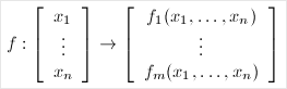
Given a function :
Given a function :
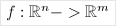
that is differentiable along both dimensions, it is possible to write f and its derivatives in the following way :
|
|
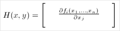
The H function is called the Jacobian matrix of f. The idea of the Newton-Raphson algorithm consists in considering that, given a point (x, y), the best direction leading to a root of the function is the direction given by the slope of f. In following this direction, the algorithm assumes that it moves closer to a root of f.
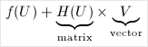
Given a vector U representing the current position, the algorithm computes f(U), a vector representing the value of f at U, as well as H(U) the Jacobian matrix of the derivatives of f at U. Now, the next position V is chosen such that:
Given a vector U representing the current position, the algorithm computes f(U), a vector representing the value of f at U, as well as H(U) the Jacobian matrix of the derivatives of f at U. Now, the next position V is chosen such that:
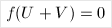
where f(U + V) is approximated by:
Then, U is replaced by U + V, and this operation is repeated until either U converges or a maximal number of iterations is reached.
1. Write the (very simple) equation linking H, U and V.
2. Write the Newton-Raphson method in a generic way:
function U = Newton_Raphson(f, J, U0, N, epsilon)
... where f is the function under study, J is its Jacobian matrix, U0 is the starting position of the algorithm, N is the maximal number of steps allowed during the algorithm and epsilon measures the convergence of the algorithm.
Remarks:
One requirement is to be able to compute the values taken by the function f and all its derivatives in a priori any point of the plane. Therefore, it is necessary to specify f and its derivatives in the form of functions. Python allows programming using functional parameters. These parameters may be provided by functions defined either with the keyword lambda, or with simple def definitions.
The algorithm requires the resolution of several linear systems with matrices M that are possibly singular, for instance such that:

Prefer the function numpy.linalg.lstsq in order to avoid such numerical problems.
One of the drawbacks of this algorithm is its tendency to diverge in numerous cases. It is therefore imperative to limit the number of steps taken, and to detect to what extent the algorithm has converged.
One of the drawbacks of this algorithm is its tendency to diverge in numerous cases. It is therefore imperative to limit the number of steps taken, and to detect to what extent the algorithm has converged.
3. Propose a very simple test protocol for a function

4. Enhance your implementation to include backtracking inside your Newton-Raphson implementation.
Computation of the Lagrangian points
Consider an object moving in the plane and subject to a set of forces. Our goal in this section consists in determining the equilibrium positions of this object.
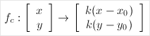
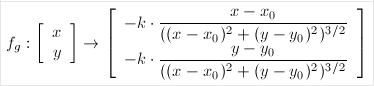
1. Write the code to represent the following kinds of forces :
1. Write the code to represent the following kinds of forces :
|
(with zero natural length)
|
Remarks:
Is is strongly recommended to use functional programming techniques to represent the forces and their Jacobian matrices.
For each of these cases, it should be possible to parameterize the force by a constant k symbolizing its intensity, as well as a central point (x0, y0) from which the force is issued.
2. Use the Newton-Raphson method to obtain the equilibrium points in the following case :
3. Is it possible to obtain the Lagrangian points?
- Two gravitational forces with respective coefficients 1 and 0.01;
- And a centrifugal force centered on the barycenter of the two masses, with coefficient 1.
3. Is it possible to obtain the Lagrangian points?
Bairstow method for polynomial factorization
Consider the problem of finding the roots of a polynomial P. When the roots of P are real, the Newton-Raphson method can be applied to find the roots. Nevertheless, this method is unable to find the complex roots of P. The Bairstow method is a method computing the irreducible factors of degree 2 of a real polynomial. Incidentally, it avoids the computations with complex numbers. Technically, it simply consists in applying the Newton-Raphson method to a specific function.
The Bairstow algorithm is described on page 377 of the Numerical Recipes available at this location (chap. 9.5 pp. 369--379).
1. Describe (literally) the function whose zero is computed in dimension 2. In particular, define its domain of definition and its range, and explain the role of the variables B, C, R and S. What are the zeros of this function ?
2. Write the code of this function by reusing the function numpy.polydiv (which computes simultaneously the quotient and the remainder of the division). In order to test this function, it suffices to construct the adequate polynomial of the form:
2. Write the code of this function by reusing the function numpy.polydiv (which computes simultaneously the quotient and the remainder of the division). In order to test this function, it suffices to construct the adequate polynomial of the form:
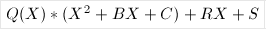
and to apply the function.
3. In the Numerical Recipes, find the 4 partial derivatives of the previous function. Write the equations defining these derivatives, and program them.
4. Write the Bairstow algorithm, and test it using a method of your choice.
3. In the Numerical Recipes, find the 4 partial derivatives of the previous function. Write the equations defining these derivatives, and program them.
4. Write the Bairstow algorithm, and test it using a method of your choice.
Electrostatic equilibrium
Let us consider the interval [-1; 1] and two electrostatic charges fixed at the positions -1 and 1. We assume that there exists N charges positioned at x1, x2, ... , xN, and that these charges can move freely in the interval [-1; 1]. The total electrostatic energy of this system is equal to:

The equilibrium positions are found by minimizing or maximizing this energy. In order to do this, it is necessary to solve a non-linear system of equations that is equal to:
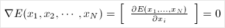
Notice that
is a vector with N coordinates.
1. Compute the Jacobian of:
1. Compute the Jacobian of:

2. Use Newton's method in order to solve this equation. Plot the points and the real axis. Do these solutions resemble to the roots of the derivative of the Legendre polynomials? (cf. numpy.polynomial.legendre)
3. Does the solution correspond to a maximum or a minimum of the energy?
3. Does the solution correspond to a maximum or a minimum of the energy?
The wave equation
When considering the propagation of waves on shallow water surfaces, a simple model is the KdV (Korteweg de Vries) equation:
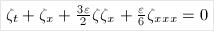
where Zeta_x denotes the derivative of Zeta with respect to x. Zeta(x, t) is the "scaled'' elevation of the surface of the wave and is a function of the time t and the space x. The true elevation is equal to h * (1 + epsilon * Zeta), the parameter epsilon will be chosen less than 1 (e.g. 0.1). We will reduce the computations on the interval and impose periodic boundary conditions.
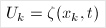
Let U be a vector of size N, discretizing Zeta on a regular subdivision:
Let U be a vector of size N, discretizing Zeta on a regular subdivision:
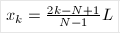
of the interval [-L; L].
We are going to compute a sequence of vector U^n representing the temporal evolution of the wave. The initial condition will be set to a Gaussian function:
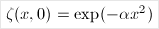
with alpha > 0
As for the heat equation, a finite difference scheme is used to solve this equation. In the following, we describe an algorithm to compute U^(n+1) as a function of U^n.
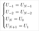
Periodic boundary conditions induce the following conditions:
As for the heat equation, a finite difference scheme is used to solve this equation. In the following, we describe an algorithm to compute U^(n+1) as a function of U^n.
Periodic boundary conditions induce the following conditions:
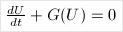
We denote G the application which transforms the vector U into the vector:

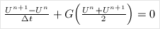
This application is non-linear and can not be represented as a matrix. We have the following evolution system:
In order to solve this evolution equation, we consider the following equation:
1. Compute and draw U^0
2. Write the function whose roots you must find. Compute the Jacobian matrix of this function.
3. Compute U^(n+1) as a function of U^n with the Newton-Raphson method. Draw the results. As an example, it should be possible to generate a movie like this one.
2. Write the function whose roots you must find. Compute the Jacobian matrix of this function.
3. Compute U^(n+1) as a function of U^n with the Newton-Raphson method. Draw the results. As an example, it should be possible to generate a movie like this one.
Analysis and conclusion
Conclude your experimentations by an analysis of the problems encountered and the benefits of using an algorithm such as the Newton-Raphson.
The comparison shall be based on the results investigated in the course, and possibly the reading of the chapter 9 of the Numerical Recipes, available at this location (chap. 9, Root Finding and Nonlinear Sets of Equations).
