Interpolation and integration methods /
Cubic splines and surface interpolation
Sujets de David Renault
This project implements a (somewhat basic) model to represent the air flow around an airfoil, i.e. the cross section of an aircraft's wing. The goal consists in obtaining a pressure map above and below the wing, so as to approximate the wing's lift, i.e. its ability to sustain the plane in the air. This is to be done in two steps: first, refine the airfoil into a sufficiently smooth curve, then compute the pressure map using integration methods.
The very first step consists in selecting an airfoil in the database of the UIUC Applied Aerodynamics Group. These data may be loaded into Python as arrays of points by using the following file.
Airfoil refinement
The airfoil consists of a list of points (defined with their abscissas and ordinates), that can be split into two parts : the upper surface of the wing (called the extrados in French) and its lower surface (called intrados). This part can be done by hand.
In order to interpolate the points of the airfoil into a sufficiently smooth curve, cubic splines are used. Points of the curve are joined by a piecewise-polynomial curve, such that each polynomial has a degree at most 3, and such that the joins between two consecutive polynomials preserve the continuity of the curve, its derivative and its second derivative.
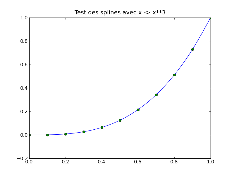
Chapter 3.3 of the Numerical Recipes describes the algorithm computing this sequence of polynomials. Here is an example of spline interpolating the points of the function x -> x^3:
In order to interpolate the points of the airfoil into a sufficiently smooth curve, cubic splines are used. Points of the curve are joined by a piecewise-polynomial curve, such that each polynomial has a degree at most 3, and such that the joins between two consecutive polynomials preserve the continuity of the curve, its derivative and its second derivative.
Chapter 3.3 of the Numerical Recipes describes the algorithm computing this sequence of polynomials. Here is an example of spline interpolating the points of the function x -> x^3:
Computing the length of plane curves
In order to approximate the pressure on either side of the airfoil, we must be able to compute the lengths of the aforementioned splines, given as function . To this purpose, we will compute a specific integral depending on the function f. As a reminder, the length of the graph of a function y = f(x) defined and differentiable on an interval [0; T] is given by the following integral:
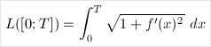
Note that it is necessary to compute the derivative of the function f, which is relatively easy when f has been interpolated by a cubic spline first.
In order to compare the results and the speeds of convergence, several integration methods must be implemented. In terms of coding, the following should be considered:
- the genericity of the functions (it must be possible to pass the integration method as a parameter)
- the efficiency of the integration method (more efficient methods perform fewer evaluations of the function f for the same level of precision)
Modeling the airflow
After having drawn the shape of our wing, the airflow is modeled around the upper and lower part. Let's suppose that the wing is currently flying in the air (or equivalently placed into a wind tunnel). The airflow is supposed to be laminar, that is to say that the airflow can be split into slices : each air molecule moves along curves that are non-intersecting, as in the following picture:
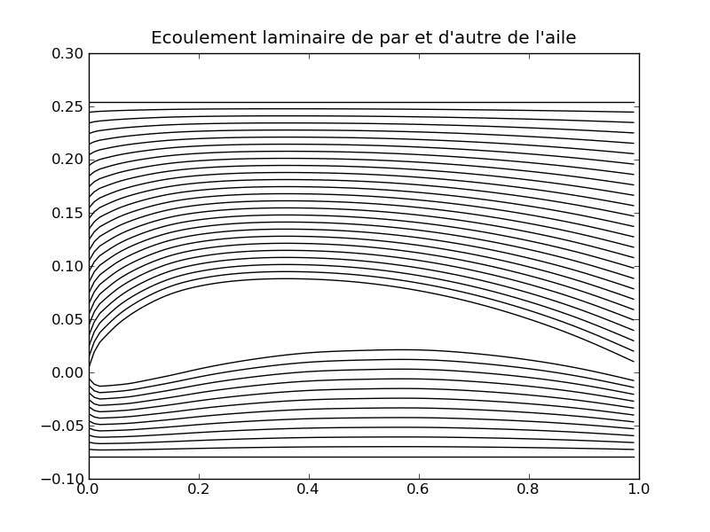
Near the airfoil, the air moves along a curve very similar to the airfoil, whereas when the air is situated further, it moves horizontally, without disturbance. The difficulty here consists in determining how the air flows between these two extreme states.
This exercise makes a number of approximations on the fluid dynamics and cannot represent the airflow in a perfectly realistic manner. Note at least that, in standard conditions, this approximation is visually acceptable.
Let (h_min resp. h_max) be the minimal (resp. maximal) height of the airfoil. In the following, we suppose that the airflow is disturbed by the wing only in a vertical interval [3h_min; 3h_max]. Out of this interval, , the air flows in a rectilinear way.
Let y = f(x) be the curve representing the upper surface of the wing. The family of curves describing the airflow above the wing are given by the following equations:
Let y = f(x) be the curve representing the upper surface of the wing. The family of curves describing the airflow above the wing are given by the following equations:

For a fixed lambda, this equation defines a curve situated between the upper side of the wing and the maximal altitude beyond which the air is not disturbed by the wing.
The pressure on each slice is computed in the following manner: the air is supposed to flow along the curves f_lambda on each part of the wing. And the air pressure as a moving fluid can be approximated with the Bernouilli Law:
The pressure on each slice is computed in the following manner: the air is supposed to flow along the curves f_lambda on each part of the wing. And the air pressure as a moving fluid can be approximated with the Bernouilli Law:
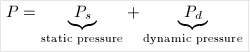
where
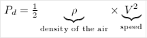
For the sake of simplicity, let's suppose that P is constant on the whole area. The variations of pressure are therefore linked to the variations of speed of the air. Since the air flows in a laminar manner, it takes the same time to pass through the zone (from the leading edge to the trailing edge of the wing), independently of the slice along which it flows. As a consequence, it is possible to compute the speed of the air as a simple function of the length of the slice.
The force induced by the air on the wing is merely due to the static pressure : it is normally weaker on the upper part of the wing than on the lower part. This difference induces a force, named the lift, that sustains the plane in the air during its flight. If we are only interested by dynamic pressure, it is possible to compute a map of this pressure around the wing that looks like the following:
The force induced by the air on the wing is merely due to the static pressure : it is normally weaker on the upper part of the wing than on the lower part. This difference induces a force, named the lift, that sustains the plane in the air during its flight. If we are only interested by dynamic pressure, it is possible to compute a map of this pressure around the wing that looks like the following:
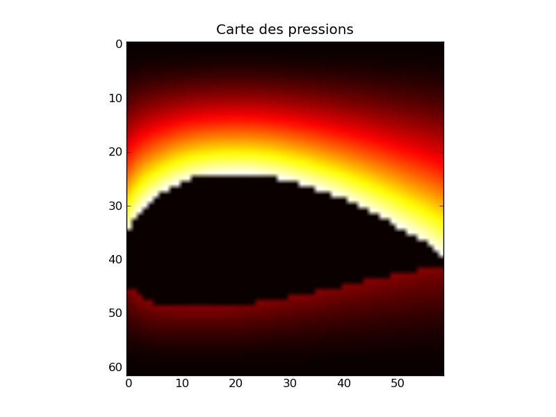
Black areas correspond to zones where the air is not disturbed, and lighter areas correspond to zones where the air must travel along a longer path. It can be notices that the air flows faster above than below.
Write a function performing the computation of a pressure map around the wing.
Write a function performing the computation of a pressure map around the wing.
